Expansion of elementary functions in a Taylor series. Maclaurin series and expansion of some functions

I’ll make a reservation right away that the article will discuss the expansion of the tangent at zero, which is called the Maclaurin expansion in many textbooks.

Well, all functions will be infinitely differentiable where we need.

While most of the other simplest elementary functions can be easily expanded into a Taylor series and the law by which the expansion terms are formed is most often not complicated and simply guessed, this is not the case for the tangent. Although it would seem that the latter is just the ratio of sine to cosine, functions with which there are no problems when decomposing. Meanwhile, in order to indicate the form of the common term for the tangent, we will have to start somewhat from afar and apply artificial methods. But, in practice, it is often not required to know all the coefficients of the series, just a few terms of the expansion are enough. With such a statement of the problem, students meet most often. So, that's where we'll start. In order not to bother especially, we will look for the decomposition up to the coefficient at the fifth degree.

The first thing that comes to mind here is to try to use Taylor's formula directly. Often, people simply do not have any idea about other ways of expanding in a row. By the way, our seminarian in mathematics. analysis, in my second year, I was looking for decomposition in this way, although I can’t say anything bad about him, the uncle is smart, maybe he just wanted to show his abilities in taking derivatives. Be that as it may, but taking high-order derivatives of the tangent pleasure is still an extremely dreary task, just one of those that is easier to entrust to a machine, and not to a person. But, we, as real athletes, are not interested in the result, but in the process, and it is desirable that the process be simpler. The derivatives are (calculated in the maxima system): , , , , . Whoever thinks that derivatives are easy to get manually, let him do it, at leisure. Anyway, now we can write out the expansion: .

To simplify here, we note that and so, the first derivative of the tangent is expressed through the tangent, in addition, it follows from this that all other derivatives of the tangent will be polynomials of the tangent, which allows us not to suffer with the derivatives of the quotient from sines and cosines:
,
,
,
.
The decomposition, of course, is the same.

I learned about another method of expansion in a series directly at the mat exam. analysis and for ignorance of this method, I then received a choir. instead of ex.-a. The meaning of the method is that we know the series expansion of both sine and cosine, as well as the function , the last expansion allows us to find the expansion of the secons: . Opening the brackets, we get a series that needs to be multiplied with the expansion of the sine. And now we just need to multiply two rows. In terms of complexity, I doubt that it is inferior to the first method, especially since the amount of computation grows rapidly as the degree of the expansion terms to be found increases.

The next method is a variant of the method of indefinite coefficients. Let us first pose the question, what do we know about the tangent from what can help us build a decomposition, so to speak a priori. The most important thing here is that the tangent function is odd, and therefore all coefficients at even powers are equal to zero, in other words, finding half of the coefficients is not required. Then you can write , or , expanding the sine and cosine into a series, we get . And equating the coefficients at the same powers, we get , , and in general . Thus, with the help of an iterative process, we can find any number of expansion terms.

The fourth method is also the method of indefinite coefficients, but for it we do not need the expansion of any other functions. We will consider the differential equation for the tangent. We saw above that the derivative of tangent can be expressed as a function of tangent. Substituting into this equation a series of indefinite coefficients, we can write . By squaring and from here, again, it will be possible to find the expansion coefficients by an iterative process.

These methods are much simpler than the first two, but finding expressions for the common member of the series in this way will not work, but we would like to. As I said at the beginning, you will have to start from afar (I will follow Courant's tutorial). We start by expanding the function into a series. As a result, we will get a series that will be written in the form , where the numbers are the Bernoulli numbers.
Initially, these numbers were found by Jacob Bernoulli when finding the sums of m-th powers of natural numbers . It would seem, and here trigonometry? Later, Euler, solving the problem of the sum of the inverse squares of a series of natural numbers, received the answer from the expansion of the sine into an infinite product. Further, it turned out that the expansion of the cotangent contains sums of the form , for all natural numbers n. And already proceeding from this, Euler obtained expressions for such sums in terms of Bernoulli numbers. So there are connections here, and one should not be surprised that the expansion of the tangent contains this sequence.
But let's get back to fraction expansion. Expanding the exponent, subtracting one and dividing by "x", we eventually get . From here it is already obvious that the first of the Bernoulli numbers is equal to one, the second minus one second, and so on. Let's write out the expression for the k-th Bernoulli number, starting from one. Multiplying this expression by , we rewrite the expression in the following form. And from this expression we can get Bernoulli numbers in turn, in particular: , ,

In the theory of functional series, the section devoted to the expansion of a function into a series occupies a central place.

Thus, the problem is posed: for a given function it is required to find such a power series

which converged on some interval and its sum was equal to
, those.

= ..

This task is called the problem of expanding a function into a power series.

A necessary condition for the expansion of a function into a power series is its differentiability an infinite number of times - this follows from the properties of convergent power series. This condition is satisfied, as a rule, for elementary functions in their domain of definition.

So let's assume that the function
has derivatives of any order. Can it be expanded into a power series, if so, how to find this series? The second part of the problem is easier to solve, so let's start with it.

Let's assume that the function
can be represented as the sum of a power series converging in an interval containing a point X 0 :

= .. (*)

where a 0 ,a 1 ,a 2 ,...,a P ,... – uncertain (yet) coefficients.

Let us put in equality (*) the value x = x 0 , then we get

.

We differentiate the power series (*) term by term

= ..

and putting here x = x 0 , we get

.

With the next differentiation, we get the series

= ..

assuming x = x 0 , we get
, where
.

After P-fold differentiation we get

Assuming in the last equality x = x 0 , we get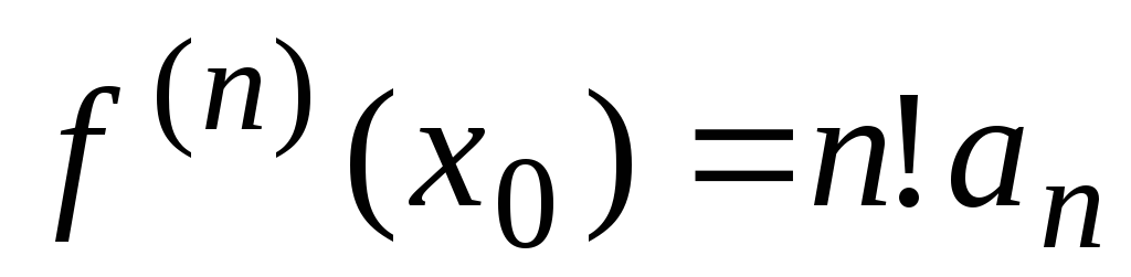
, where

So the coefficients are found

,
,
, …,
,….,

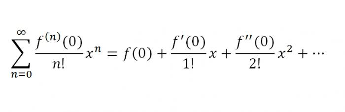
substituting which into a row (*), we get

The resulting series is called near taylor for function
.

Thus, we have established that if the function can be expanded into a power series in powers (x - x 0 ), then this expansion is unique and the resulting series is necessarily a Taylor series.

Note that the Taylor series can be obtained for any function that has derivatives of any order at the point x = x 0 . But this does not yet mean that an equal sign can be put between the function and the resulting series, i.e. that the sum of the series is equal to the original function. Firstly, such an equality can only make sense in the region of convergence, and the Taylor series obtained for the function may diverge, and secondly, if the Taylor series converges, then its sum may not coincide with the original function.

3.2. Sufficient conditions for the expansion of a function into a Taylor series

Let us formulate a statement with the help of which the stated problem will be solved.

If the function
in some neighborhood of the point x 0 has derivatives up to (n+ 1)-th order inclusive, then in this neighborhood we haveformula Taylor

whereR n (X)-residual term of the Taylor formula - has the form (Lagrange form)

where dotξ lies between x and x 0 .

Note that there is a difference between the Taylor series and the Taylor formula: the Taylor formula is a finite sum, i.e. P - fixed number.

Recall that the sum of the series S(x) can be defined as the limit of the functional sequence of partial sums S P (x) at some interval X:

.

According to this, to expand a function into a Taylor series means to find a series such that for any XX

We write the Taylor formula in the form where

notice, that
defines the error we get, replace the function f(x) polynomial S n (x).

If a
, then
,those. the function expands into a Taylor series. Conversely, if
, then
.

Thus, we have proved criterion for the expansion of a function into a Taylor series.

In order that in some interval the functionf(x) expands in a Taylor series, it is necessary and sufficient that on this interval
, whereR n (x) is the remainder of the Taylor series.

With the help of the formulated criterion, one can obtain sufficientconditions for the expansion of a function into a Taylor series.

If insome neighborhood of the point x 0 the absolute values ​​of all derivatives of a function are limited by the same number M≥ 0, i.e.

, to in this neighborhood, the function expands into a Taylor series.

From the above it follows algorithmfunction expansion f(x) in a Taylor series in the vicinity of the point X 0 :

1. Finding derivative functions f(x):

f(x), f’(x), f”(x), f’”(x), f (n) (x),…

2. We calculate the value of the function and the values ​​of its derivatives at the point X 0

f(x 0 ), f'(x 0 ), f”(x 0 ), f’”(x 0 ), f (n) (x 0 ),…

3. We formally write the Taylor series and find the region of convergence of the resulting power series.

4. We check the fulfillment of sufficient conditions, i.e. establish for which X from the convergence region, remainder term R n (x) tends to zero at
or
.

The expansion of functions in a Taylor series according to this algorithm is called expansion of a function in a Taylor series by definition or direct decomposition.

If the function f(x) has on some interval containing a point a, derivatives of all orders, then the Taylor formula can be applied to it:

where rn- the so-called residual term or the remainder of the series, it can be estimated using the Lagrange formula:

, where the number x is enclosed between X and a.

If for some value x r n®0 at n®¥, then in the limit the Taylor formula for this value turns into a convergent formula Taylor series:

So the function f(x) can be expanded into a Taylor series at the considered point X, if:

1) it has derivatives of all orders;

2) the constructed series converges at this point.

At a=0 we get a series called near Maclaurin:

Example 1 f(x)= 2x.

Decision. Let us find the values ​​of the function and its derivatives at X=0

f(x) = 2x, f( 0) = 2 0 =1;

f¢(x) = 2x ln2, f¢( 0) = 2 0 ln2=ln2;

f¢¢(x) = 2x ln 2 2, f¢¢( 0) = 2 0 log 2 2= log 2 2;

f(n)(x) = 2x ln n 2, f(n)( 0) = 2 0 ln n 2=ln n 2.

Substituting the obtained values ​​of the derivatives into the Taylor series formula, we get:

The radius of convergence of this series is equal to infinity, so this expansion is valid for -¥<x<+¥.

Example 2 X+4) for the function f(x)= e x.

Decision. Finding the derivatives of the function e x and their values ​​at the point X=-4.

f(x)= e x, f(-4) = e -4 ;

f¢(x)= e x, f¢(-4) = e -4 ;

f¢¢(x)= e x, f¢¢(-4) = e -4 ;

f(n)(x)= e x, f(n)( -4) = e -4 .

Therefore, the desired Taylor series of the function has the form:

This decomposition is also valid for -¥<x<+¥.

Example 3 . Expand function f(x)=ln x in a series by degrees ( X- 1),

(i.e. in a Taylor series in the vicinity of the point X=1).

Decision. We find the derivatives of this function.

Substituting these values ​​into the formula, we get the desired Taylor series:

With the help of d'Alembert's test, one can verify that the series converges when

½ X- 1½<1. Действительно,

The series converges if ½ X- 1½<1, т.е. при 0<x<2. При X=2 we obtain an alternating series that satisfies the conditions of the Leibniz test. At X=0 function is not defined. Thus, the region of convergence of the Taylor series is the half-open interval (0;2].

Let us present the expansions obtained in this way in the Maclaurin series (i.e., in a neighborhood of the point X=0) for some elementary functions:

(2) ,

(3) ,

( the last expansion is called binomial series)

Example 4 . Expand the function into a power series

Decision. In decomposition (1), we replace X on the - X 2 , we get:

Example 5 . Expand the function in a Maclaurin series

Decision. We have

Using formula (4), we can write:

substituting instead of X into the formula -X, we get:

From here we find:

Expanding the brackets, rearranging the terms of the series and making a reduction of similar terms, we get

This series converges in the interval

(-1;1) since it is derived from two series, each of which converges in this interval.

Comment .

Formulas (1)-(5) can also be used to expand the corresponding functions in a Taylor series, i.e. for the expansion of functions in positive integer powers ( Ha). To do this, it is necessary to perform such identical transformations on a given function in order to obtain one of the functions (1) - (5), in which instead of X costs k( Ha) m , where k is a constant number, m is a positive integer. It is often convenient to change the variable t=Ha and expand the resulting function with respect to t in the Maclaurin series.

This method illustrates the theorem on the uniqueness of the expansion of a function in a power series. The essence of this theorem is that in the neighborhood of the same point, two different power series cannot be obtained that would converge to the same function, no matter how its expansion is performed.

Example 6 . Expand the function in a Taylor series in a neighborhood of a point X=3.

Decision. This problem can be solved, as before, using the definition of the Taylor series, for which it is necessary to find the derivatives of the functions and their values ​​at X=3. However, it will be easier to use the existing decomposition (5):

The resulting series converges at or -3<x- 3<3, 0<x< 6 и является искомым рядом Тейлора для данной функции.

Example 7 . Write a Taylor series in powers ( X-1) features .

Decision.

The series converges at , or 2< x£5.

Students of higher mathematics should be aware that the sum of a certain power series belonging to the interval of convergence of the series given to us turns out to be a continuous and unlimited number of times differentiated function. The question arises: is it possible to assert that a given arbitrary function f(x) is the sum of some power series? That is, under what conditions can the function f(x) be represented by a power series? The importance of this question lies in the fact that it is possible to approximately replace the function f(x) by the sum of the first few terms of the power series, that is, by a polynomial. Such a replacement of a function by a rather simple expression - a polynomial - is also convenient when solving some problems, namely: when solving integrals, when calculating, etc.

It is proved that for some function f(x), in which derivatives up to the (n + 1)th order, including the last one, can be calculated, in the neighborhood (α - R; x 0 + R) of some point x = α formula:

This formula is named after the famous scientist Brook Taylor. The series that is obtained from the previous one is called the Maclaurin series:

The rule that makes it possible to expand in a Maclaurin series:

1. Determine the derivatives of the first, second, third ... orders.
2. Calculate what the derivatives at x=0 are.
3. Write the Maclaurin series for this function, and then determine the interval of its convergence.
4. Determine the interval (-R;R), where the remainder of the Maclaurin formula

R n (x) -> 0 for n -> infinity. If one exists, the function f(x) in it must coincide with the sum of the Maclaurin series.

Consider now the Maclaurin series for individual functions.

1. So, the first will be f(x) = e x. Of course, according to its features, such a function has derivatives of very different orders, and f (k) (x) \u003d e x, where k equals everything Let us substitute x \u003d 0. We get f (k) (0) \u003d e 0 \u003d 1, k \u003d 1.2 ... Based on the foregoing, the series e x will look like this:

2. Maclaurin series for the function f(x) = sin x. Immediately clarify that the function for all unknowns will have derivatives, besides f "(x) \u003d cos x \u003d sin (x + n / 2), f "" (x) \u003d -sin x \u003d sin (x +2*n/2)..., f(k)(x)=sin(x+k*n/2), where k is equal to any natural number.That is, by making simple calculations, we can conclude that the series for f(x) = sin x will look like this:

3. Now let's try to consider the function f(x) = cos x. It has derivatives of arbitrary order for all unknowns, and |f (k) (x)| = |cos(x+k*n/2)|<=1, k=1,2... Снова-таки, произведя определенные расчеты, получим, что ряд для f(х) = cos х будет выглядеть так:

So, we have listed the most important functions that can be expanded in the Maclaurin series, but they are supplemented by Taylor series for some functions. Now we will list them. It is also worth noting that Taylor and Maclaurin series are an important part of the practice of solving series in higher mathematics. So, Taylor series.

1. The first will be a row for f-ii f (x) = ln (1 + x). As in the previous examples, given us f (x) = ln (1 + x), we can add a series using the general form of the Maclaurin series. however, for this function, the Maclaurin series can be obtained much more simply. After integrating a certain geometric series, we get a series for f (x) = ln (1 + x) of such a sample:

2. And the second, which will be final in our article, will be a series for f (x) \u003d arctg x. For x belonging to the interval [-1; 1], the expansion is valid:

That's all. In this article, the most used Taylor and Maclaurin series in higher mathematics, in particular, in economic and technical universities, were considered.

16.1. Expansion of elementary functions in Taylor series and

Maclaurin

Let us show that if an arbitrary function is defined on the set
, in the vicinity of the point
has many derivatives and is the sum of a power series:

then you can find the coefficients of this series.

Substitute in a power series
. Then
.

Find the first derivative of the function
:

At
:
.

For the second derivative we get:

At
:
.

Continuing this procedure n once we get:
.

Thus, we got a power series of the form:

,

which is called near taylor for function
around the point
.

A special case of the Taylor series is Maclaurin series at
:

The remainder of the Taylor (Maclaurin) series is obtained by discarding the main series n the first terms and is denoted as
. Then the function
can be written as a sum n the first members of the series
and the remainder
:,

.

The rest is usually
expressed in different formulas.

One of them is in the Lagrange form:

, where
.
.

Note that in practice the Maclaurin series is used more often. Thus, in order to write the function
in the form of a sum of a power series, it is necessary:

1) find the coefficients of the Maclaurin (Taylor) series;

2) find the region of convergence of the resulting power series;

3) prove that the given series converges to the function
.

Theorem1 (a necessary and sufficient condition for the convergence of the Maclaurin series). Let the convergence radius of the series
. In order for this series to converge in the interval
to function
, it is necessary and sufficient that the following condition is satisfied:
within the specified interval.

Theorem 2. If derivatives of any order of a function
in some interval
limited in absolute value to the same number M, i.e
, then in this interval the function
can be expanded in a Maclaurin series.

Example1 . Expand in a Taylor series around the point
function.

Decision.

.

,;

,
;

,
;

,

.......................................................................................................................................

,
;

Convergence area
.

Example2 . Expand function in a Taylor series around a point
.

Decision:

We find the value of the function and its derivatives at
.

,
;

,
;

...........……………………………

,
.

Substitute these values ​​in a row. We get:

or
.

Let us find the region of convergence of this series. According to the d'Alembert test, the series converges if

.

Therefore, for any this limit is less than 1, and therefore the area of ​​convergence of the series will be:
.

Let us consider several examples of the expansion into the Maclaurin series of basic elementary functions. Recall that the Maclaurin series:

.

converges on the interval
to function
.

Note that to expand the function into a series, it is necessary:

a) find the coefficients of the Maclaurin series for a given function;

b) calculate the radius of convergence for the resulting series;

c) prove that the resulting series converges to the function
.

Example 3 Consider the function
.

Decision.

Let us calculate the value of the function and its derivatives for
.

Then the numerical coefficients of the series have the form:

for anyone n. We substitute the found coefficients in the Maclaurin series and get:

Find the radius of convergence of the resulting series, namely:

.

Therefore, the series converges on the interval
.

This series converges to the function for any values , because on any interval
function and its absolute value derivatives are limited by the number .

Example4 . Consider the function
.

Decision.

:

It is easy to see that even-order derivatives
, and derivatives of odd order. We substitute the found coefficients in the Maclaurin series and get the expansion:

Let us find the interval of convergence of this series. According to d'Alembert:

for anyone . Therefore, the series converges on the interval
.

This series converges to the function
, because all its derivatives are limited to one.

Example5 .
.

Decision.

Let us find the value of the function and its derivatives at
:

Thus, the coefficients of this series:
and
, hence:

Similarly with the previous series, the area of ​​convergence
. The series converges to the function
, because all its derivatives are limited to one.

Note that the function
odd and series expansion in odd powers, function
– even and expansion in a series in even powers.

Example6 . Binomial series:
.

Decision.

Let us find the value of the function and its derivatives at
:

This shows that:

We substitute these values ​​of the coefficients in the Maclaurin series and obtain the expansion of this function in a power series:

Let's find the radius of convergence of this series:

Therefore, the series converges on the interval
. At the limit points at
and
series may or may not converge depending on the exponent
.

The studied series converges on the interval
to function
, that is, the sum of the series
at
.

Example7 . Let us expand the function in a Maclaurin series
.

Decision.

To expand this function into a series, we use the binomial series for
. We get:

Based on the property of power series (a power series can be integrated in the region of its convergence), we find the integral of the left and right parts of this series:

Find the area of ​​convergence of this series:
,

that is, the convergence region of this series is the interval
. Let us determine the convergence of the series at the ends of the interval. At

. This series is a harmonic series, that is, it diverges. At
we get a number series with a common term
.

The Leibniz series converges. Thus, the region of convergence of this series is the interval
.

16.2. Application of power series of powers in approximate calculations

Power series play an extremely important role in approximate calculations. With their help, tables of trigonometric functions, tables of logarithms, tables of values ​​of other functions that are used in various fields of knowledge, for example, in probability theory and mathematical statistics, were compiled. In addition, the expansion of functions in a power series is useful for their theoretical study. The main issue when using power series in approximate calculations is the question of estimating the error when replacing the sum of a series by the sum of its first n members.

Consider two cases:

the function is expanded into an alternating series;

the function is expanded into a constant-sign series.

Calculation using alternating series

Let the function
expanded into an alternating power series. Then, when calculating this function for a specific value we get a number series to which we can apply the Leibniz test. In accordance with this criterion, if the sum of a series is replaced by the sum of its first n members, then the absolute error does not exceed the first term of the remainder of this series, that is:
.

Example8 . Calculate
with an accuracy of 0.0001.

Decision.

We will use the Maclaurin series for
, substituting the value of the angle in radians:

If we compare the first and second members of the series with a given accuracy, then: .

Third expansion term:

less than the specified calculation accuracy. Therefore, to calculate
it suffices to leave two terms of the series, i.e.

.

Thus
.

Example9 . Calculate
with an accuracy of 0.001.

Decision.

We will use the binomial series formula. For this we write
as:
.

In this expression
,

Let's compare each of the terms of the series with the accuracy that is given. It's clear that
. Therefore, to calculate
it suffices to leave three members of the series.

or
.

Calculation using sign-positive series

Example10 . Calculate number with an accuracy of 0.001.

Decision.

In a row for a function
substitute
. We get:

Let us estimate the error that arises when the sum of the series is replaced by the sum of the first members. Let's write down the obvious inequality:

i.e. 2<<3. Используем формулу остаточного члена ряда в форме Лагранжа:
,
.

According to the condition of the problem, you need to find n such that the following inequality holds:
or
.

It is easy to check that when n= 6:
.

Hence,
.

Example11 . Calculate
with an accuracy of 0.0001.

Decision.

Note that to calculate the logarithms, one could apply the series for the function
, but this series converges very slowly and 9999 terms would have to be taken to achieve the given accuracy! Therefore, to calculate logarithms, as a rule, a series for the function is used
, which converges on the interval
.

Compute
with this row. Let be
, then .

Hence,
,

In order to calculate
with a given accuracy, take the sum of the first four terms:
.

The rest of the row
discard. Let's estimate the error. It's obvious that

or
.

Thus, in the series that was used for the calculation, it was enough to take only the first four terms instead of 9999 in the series for the function
.

Questions for self-diagnosis

1. What is a Taylor series?

2. what kind of series did Maclaurin have?

3. Formulate a theorem on the expansion of a function in a Taylor series.

4. Write the expansion in the Maclaurin series of the main functions.

5. Indicate the areas of convergence of the considered series.

6. How to estimate the error in approximate calculations using power series?