Confidence intervals. Confidence interval

And others. All of them are estimates of their theoretical analogues, which could be obtained if not a sample, but a general population were available. But alas, the general population is very expensive and often inaccessible.

The concept of interval estimation

Any sample estimate has some spread, because is a random variable depending on the values ​​in a particular sample. Therefore, for more reliable statistical conclusions, one should know not only the point estimate, but also the interval, which with a high probability γ (gamma) covers the evaluated indicator θ (theta).

Formally, these are two such values ​​(statistics) T 1 (X) And T 2 (X), What T 1< T 2 , for which at a given probability level γ the condition is met:

In short, it is likely γ or more the true indicator is between the points T 1 (X) And T 2 (X), which are called the lower and upper bounds confidence interval.

One of the conditions for constructing confidence intervals is its maximum narrowness, i.e. it should be as short as possible. The desire is quite natural, because... the researcher tries to more accurately localize the location of the desired parameter.

It follows that the confidence interval must cover the maximum probabilities of the distribution. and the assessment itself should be in the center.

That is, the probability of deviation (of the true indicator from the estimate) upward is equal to the probability of deviation downward. It should also be noted that for asymmetric distributions, the interval on the right is not equal to the interval on the left.

The figure above clearly shows that the greater the confidence probability, the wider the interval - a direct relationship.

This was a short introduction to the theory of interval estimation of unknown parameters. Let's move on to finding confidence limits for the mathematical expectation.

Confidence interval for mathematical expectation

If the original data are distributed over , then the average will be a normal value. This follows from the rule that a linear combination of normal values ​​also has a normal distribution. Therefore, to calculate probabilities we could use the mathematical apparatus of the normal distribution law.

However, this will require knowing two parameters - expectation and variance, which are usually unknown. You can, of course, use estimates instead of parameters (arithmetic mean and ), but then the distribution of the average will not be entirely normal, it will be slightly flattened downward. This fact was cleverly noted by citizen William Gosset from Ireland, publishing his discovery in the March 1908 issue of the journal Biometrica. For purposes of secrecy, Gosset signed himself Student. This is how the Student t-distribution appeared.

However, the normal distribution of data, used by K. Gauss in analyzing errors in astronomical observations, is extremely rare in earthly life and is quite difficult to establish (about 2 thousand observations are needed for high accuracy). Therefore, it is best to discard the assumption of normality and use methods that do not depend on the distribution of the original data.

The question arises: what is the distribution of the arithmetic mean if it is calculated from the data of an unknown distribution? The answer is given by the well-known in probability theory Central limit theorem(CPT). In mathematics, there are several variants of it (the formulations have been refined over the years), but all of them, roughly speaking, boil down to the statement that the sum of a large number of independent random variables obeys the normal distribution law.

When calculating the arithmetic mean, the sum of random variables is used. From here it turns out that the arithmetic mean has a normal distribution, in which the expectation is the expectation of the original data, and the variance is .

Smart people know how to prove CLT, but we will verify this with the help of an experiment conducted in Excel. Let's simulate a sample of 50 uniformly distributed random variables (using the Excel function RANDBETWEEN). Then we will make 1000 such samples and calculate the arithmetic mean for each. Let's look at their distribution.

It can be seen that the distribution of the average is close to the normal law. If the sample size and number are made even larger, the similarity will be even better.

Now that we have seen with our own eyes the validity of the CLT, we can, using , calculate confidence intervals for the arithmetic mean, which cover the true mean or mathematical expectation with a given probability.

To establish the upper and lower limits, you need to know the parameters of the normal distribution. As a rule, there are none, so estimates are used: arithmetic mean And sample variance. I repeat, this method gives a good approximation only with large samples. When samples are small, it is often recommended to use the Student distribution. Don't believe it! The Student distribution for the mean occurs only when the original data is normally distributed, that is, almost never. Therefore, it is better to immediately set a minimum bar for the amount of required data and use asymptotically correct methods. They say 30 observations are enough. Take 50 - you won't go wrong.

T 1.2– lower and upper limits of the confidence interval

– sample arithmetic mean

s 0– standard deviation of the sample (unbiased)

n – sample size

γ – confidence probability (usually equal to 0.9, 0.95 or 0.99)

c γ =Φ -1 ((1+γ)/2)– the inverse value of the standard normal distribution function. Simply put, this is the number of standard errors from the arithmetic mean to the lower or upper bound (these three probabilities correspond to values ​​of 1.64, 1.96 and 2.58).

The essence of the formula is that the arithmetic mean is taken and then a certain amount is set aside from it ( with γ) standard errors ( s 0 /√n). Everything is known, take it and consider it.

Before the widespread use of personal computers, they used to obtain the values ​​of the normal distribution function and its inverse. They are still used today, but it is more effective to use ready-made Excel formulas. All elements from the formula above ( , and ) can be easily calculated in Excel. But there is a ready-made formula for calculating the confidence interval - TRUST.NORM. Its syntax is as follows.

CONFIDENCE.NORM(alpha;standard_off;size)

alpha– significance level or confidence level, which in the notation adopted above is equal to 1- γ, i.e. the probability that the mathematicalthe expectation will be outside the confidence interval. With a confidence level of 0.95, alpha is 0.05, etc.

standard_off– standard deviation of sample data. There is no need to calculate the standard error; Excel itself will divide by the root of n.

size– sample size (n).

The result of the CONFIDENCE NORM function is the second term from the formula for calculating the confidence interval, i.e. half-interval Accordingly, the lower and upper points are the average ± the obtained value.

Thus, it is possible to construct a universal algorithm for calculating confidence intervals for the arithmetic mean, which does not depend on the distribution of the original data. The price for universality is its asymptotic nature, i.e. the need to use relatively large samples. However, in the age of modern technology, collecting the required amount of data is usually not difficult.

Testing statistical hypotheses using confidence intervals

(module 111)

One of the main problems solved in statistics is. Its essence is briefly as follows. An assumption is made, for example, that the expectation of the general population is equal to some value. Then the distribution of sample means that can be observed for a given expectation is constructed. Next, they look at where in this conditional distribution the real average is located. If it goes beyond acceptable limits, then the appearance of such an average is very unlikely, and if the experiment is repeated once, it is almost impossible, which contradicts the hypothesis put forward, which is successfully rejected. If the average does not go beyond the critical level, then the hypothesis is not rejected (but also not proven!).

So, with the help of confidence intervals, in our case for expectation, you can also test some hypotheses. It's very easy to do. Let's say the arithmetic mean for a certain sample is equal to 100. The hypothesis is tested that the expected value is, say, 90. That is, if we pose the question primitively, it sounds like this: can it be that with the true value of the mean equal to 90, the observed the average turned out to be 100?

To answer this question, you will additionally need information about standard deviation and sample size. Let's assume the standard deviation is 30 and the number of observations is 64 (to easily extract the root). Then the standard error of the mean is 30/8 or 3.75. To calculate a 95% confidence interval, you will need to add two standard errors to each side of the mean (more precisely, 1.96). The confidence interval will be approximately 100±7.5 or from 92.5 to 107.5.

Further reasoning is as follows. If the value being tested falls within the confidence interval, then it does not contradict the hypothesis, because falls within the limits of random fluctuations (with a probability of 95%). If the point being checked falls outside the confidence interval, then the probability of such an event is very small, in any case below the acceptable level. This means that the hypothesis is rejected as contradicting the observed data. In our case, the hypothesis about the expected value is outside the confidence interval (the tested value of 90 is not included in the interval 100±7.5), so it should be rejected. Answering the primitive question above, it should be said: no, it cannot, in any case, this happens extremely rarely. Often, they indicate the specific probability of erroneously rejecting the hypothesis (p-level), and not the specified level on which the confidence interval was constructed, but more on that another time.

As you can see, constructing a confidence interval for the average (or mathematical expectation) is not difficult. The main thing is to grasp the essence, and then things will move on. In practice, most cases use a 95% confidence interval, which is approximately two standard errors wide on either side of the mean.

That's all for now. All the best!

Estimation of Confidence Intervals

Statistics consider the following two main tasks:

We have some estimate based on sample data, and we want to make some probabilistic statement about where the true value of the estimated parameter lies.

We have a specific hypothesis that needs to be tested using sample data.

In this topic we consider the first task. Let us also introduce the definition of a confidence interval.

After studying the material on this topic, you:

learn what a confidence interval is for an estimate;

learn to classify statistical problems;

master the technique of constructing confidence intervals, both using statistical formulas and using software tools;

learn to determine the required sample sizes to achieve certain parameters of accuracy of statistical estimates.

Distributions of sample characteristics

As discussed above, the distribution of the random variable is close to the standardized normal distribution with parameters 0 and 1. Since we do not know the value of σ, we replace it with some estimate of s. The quantity already has a different distribution, namely or Student distribution, which is determined by the parameter n -1 (the number of degrees of freedom). This distribution is close to the normal distribution (the larger n, the closer the distributions).

In Fig. 95
the Student distribution with 30 degrees of freedom is presented. As you can see, it is very close to the normal distribution.

Similar to the functions for working with the normal distribution NORMIDIST and NORMINV, there are functions for working with the t-distribution - STUDIST (TDIST) and STUDRASOBR (TINV). An example of using these functions can be seen in the file STUDRASP.XLS (template and solution) and in Fig. 96
.

As we already know, to determine the accuracy of estimating the mathematical expectation, we need a t-distribution. To estimate other parameters, such as variance, different distributions are required. Two of them are the F-distribution and x 2 -distribution.

Confidence interval for the mean

Confidence interval- this is an interval that is built around the estimated value of the parameter and shows where the true value of the estimated parameter is located with an a priori specified probability.

The construction of a confidence interval for the average value occurs in the following way:

Example

The fast food restaurant plans to expand its assortment with a new type of sandwich. In order to estimate the demand for it, the manager plans to randomly select 40 visitors from those who have already tried it and ask them to rate their attitude towards the new product on a scale from 1 to 10. The manager wants to estimate the expected number of points that the new product will receive and construct a 95% confidence interval for this estimate. How to do this? (see file SANDWICH1.XLS (template and solution).

Solution

To solve this problem you can use . The results are presented in Fig. 97
.

Confidence interval for total value

Sometimes, using sample data, it is necessary to estimate not the mathematical expectation, but the total sum of values. For example, in a situation with an auditor, the interest may be in estimating not the average account size, but the sum of all accounts.

Let N be the total number of elements, n be the sample size, T 3 be the sum of the values ​​in the sample, T" be the estimate for the sum of the entire population, then , and the confidence interval is calculated by the formula , where s is the estimate of the standard deviation for the sample, and is the estimate of the mean for the sample.

Example

Let's say a tax agency wants to estimate the total tax refunds for 10,000 taxpayers. The taxpayer either receives a refund or pays additional taxes. Find the 95% confidence interval for the refund amount, assuming a sample size of 500 people (see the file AMOUNT OF REFUND.XLS (template and solution).

Solution

StatPro does not have a special procedure for this case, however, it can be noted that the boundaries can be obtained from the boundaries for the average based on the above formulas (Fig. 98
).

Confidence interval for proportion

Let p be the mathematical expectation of the share of clients, and let p b be the estimate of this share obtained from a sample of size n. It can be shown that for sufficiently large the assessment distribution will be close to normal with mathematical expectation p and standard deviation . The standard error of estimation in this case is expressed as , and the confidence interval is as .

Example

The fast food restaurant plans to expand its assortment with a new type of sandwich. In order to assess the demand for it, the manager randomly selected 40 visitors from those who had already tried it and asked them to rate their attitude towards the new product on a scale from 1 to 10. The manager wants to estimate the expected proportion of customers who rate the new product at least than 6 points (he expects that these customers will be the consumers of the new product).

Solution

Initially, we create a new column based on attribute 1 if the client’s rating was more than 6 points and 0 otherwise (see file SANDWICH2.XLS (template and solution).

Method 1

By counting the number of 1, we estimate the share, and then use the formulas.

The zcr value is taken from special normal distribution tables (for example, 1.96 for a 95% confidence interval).

Using this approach and specific data to construct a 95% interval, we obtain the following results (Fig. 99
). The critical value of the parameter zcr is 1.96. The standard error of the estimate is 0.077. The lower limit of the confidence interval is 0.475. The upper limit of the confidence interval is 0.775. Thus, the manager has the right to believe with 95% confidence that the percentage of customers who rate the new product 6 points or higher will be between 47.5 and 77.5.

Method 2

This problem can be solved using standard StatPro tools. To do this, it is enough to note that the share in this case coincides with the average value of the Type column. Next we apply StatPro/Statistical Inference/One-Sample Analysis to construct a confidence interval of the mean (estimate of the mathematical expectation) for the Type column. The results obtained in this case will be very close to the results of the 1st method (Fig. 99).

Confidence interval for standard deviation

s is used as an estimate of the standard deviation (the formula is given in Section 1). The density function of the estimate s is the chi-square function, which, like the t-distribution, has n-1 degrees of freedom. There are special functions for working with this distribution CHIDIST and CHIINV.

The confidence interval in this case will no longer be symmetrical. A conventional boundary diagram is shown in Fig. 100 .

Example

The machine must produce parts with a diameter of 10 cm. However, due to various circumstances, errors occur. The quality controller is concerned about two circumstances: firstly, the average value should be 10 cm; secondly, even in this case, if the deviations are large, then many parts will be rejected. Every day he makes a sample of 50 parts (see file QUALITY CONTROL.XLS (template and solution). What conclusions can such a sample give?

Solution

Let's construct 95% confidence intervals for the mean and standard deviation using StatPro/Statistical Inference/One-Sample Analysis(Fig. 101
).

Next, using the assumption of a normal distribution of diameters, we calculate the proportion of defective products, setting a maximum deviation of 0.065. Using the capabilities of the substitution table (the case of two parameters), we plot the dependence of the proportion of defects on the average value and standard deviation (Fig. 102
).

Confidence interval for the difference between two means

This is one of the most important applications of statistical methods. Examples of situations.

A clothing store manager would like to know how much more or less the average female customer spends in the store than the average male customer.

The two airlines fly similar routes. A consumer organization would like to compare the difference between the average expected flight delay times for both airlines.

The company sends out coupons for certain types of goods in one city and not in another. Managers want to compare the average purchase volumes of these products over the next two months.

A car dealer often deals with married couples at presentations. To understand their personal reactions to the presentation, couples are often interviewed separately. The manager wants to evaluate the difference in the ratings given by men and women.

Case of independent samples

The difference between the means will have a t-distribution with n 1 + n 2 - 2 degrees of freedom. The confidence interval for μ 1 - μ 2 is expressed by the relation:

This problem can be solved not only using the above formulas, but also using standard StatPro tools. To do this, it is enough to use

Confidence interval for the difference between proportions

Let be the mathematical expectation of shares. Let be their sample estimates, constructed from samples of size n 1 and n 2, respectively. Then is an estimate for the difference . Therefore, the confidence interval of this difference is expressed as:

Here z cr is a value obtained from a normal distribution using special tables (for example, 1.96 for a 95% confidence interval).

The standard error of estimation is expressed in this case by the relation:

.

Example

The store, preparing for a big sale, undertook the following marketing research. The top 300 buyers were selected and randomly divided into two groups of 150 members each. All selected buyers were sent invitations to participate in the sale, but only members of the first group received a coupon entitling them to a 5% discount. During the sale, the purchases of all 300 selected buyers were recorded. How can a manager interpret the results and make a judgment about the effectiveness of coupons? (see file COUPONS.XLS (template and solution)).

Solution

For our specific case, out of 150 customers who received a discount coupon, 55 made a purchase on sale, and among the 150 who did not receive a coupon, only 35 made a purchase (Fig. 103
). Then the values ​​of the sample proportions are 0.3667 and 0.2333, respectively. And the sample difference between them is equal to 0.1333, respectively. Assuming a 95% confidence interval, we find from the normal distribution table z cr = 1.96. The calculation of the standard error of the sample difference is 0.0524. We finally find that the lower limit of the 95% confidence interval is 0.0307, ​​and the upper limit is 0.2359, respectively. The results obtained can be interpreted in such a way that for every 100 customers who received a discount coupon, we can expect from 3 to 23 new customers. However, we must keep in mind that this conclusion in itself does not mean the effectiveness of using coupons (since by providing a discount, we lose profit!). Let's demonstrate this with specific data. Let's assume that the average purchase size is 400 rubles, of which 50 rubles. there is a profit for the store. Then the expected profit on 100 customers who did not receive a coupon is:

50 0.2333 100 = 1166.50 rub.

Similar calculations for 100 customers who received a coupon give:

30 0.3667 100 = 1100.10 rub.

The decrease in average profit to 30 is explained by the fact that, using the discount, customers who received a coupon will on average make a purchase for 380 rubles.

Thus, the final conclusion indicates the ineffectiveness of using such coupons in this particular situation.

Comment. This problem can be solved using standard StatPro tools. To do this, it is enough to reduce this problem to the problem of estimating the difference between two averages using the method, and then apply StatPro/Statistical Inference/Two-Sample Analysis to construct a confidence interval for the difference between two average values.

Controlling the Confidence Interval Length

The length of the confidence interval depends on following conditions:

data directly (standard deviation);

level of significance;

sample size.

Sample size for estimating mean

First, let's consider the problem in the general case. Let us denote the value of half the length of the confidence interval given to us as B (Fig. 104
). We know that the confidence interval for the mean value of some random variable X is expressed as , Where . Believing:

and expressing n, we get .

Unfortunately, we do not know the exact value of the variance of the random variable X. In addition, we do not know the value of tcr, since it depends on n through the number of degrees of freedom. In this situation, we can do the following. Instead of variance s, we use some estimate of the variance based on any available implementations of the random variable under study. Instead of the t cr value, we use the z cr value for the normal distribution. This is quite acceptable, since the distribution density functions for the normal and t-distributions are very close (except for the case of small n). Thus, the required formula takes the form:

.

Since the formula gives, generally speaking, non-integer results, rounding with an excess of the result is taken as the desired sample size.

Example

The fast food restaurant plans to expand its assortment with a new type of sandwich. In order to assess the demand for it, the manager plans to randomly select a number of visitors from those who have already tried it and ask them to rate their attitude towards the new product on a scale from 1 to 10. The manager wants to estimate the expected number of points that the new product will receive product and construct a 95% confidence interval for this estimate. At the same time, he wants the half-width of the confidence interval to not exceed 0.3. How many visitors does he need to interview?

as follows:

Here r ots is an estimate of the proportion p, and B is a given half the length of the confidence interval. An overestimate for n can be obtained using the value r ots= 0.5. In this case, the length of the confidence interval will not exceed the specified value B for any true value of p.

Example

Let the manager from the previous example plan to estimate the share of customers who preferred a new type of product. He wants to construct a 90% confidence interval whose half length does not exceed 0.05. How many clients should be included in the random sample?

Solution

In our case, the value of z cr = 1.645. Therefore, the required quantity is calculated as .

If the manager had reason to believe that the desired p-value was, for example, approximately 0.3, then by substituting this value into the above formula, we would get a smaller random sample value, namely 228.

Formula for determining random sample size in case of difference between two means written as:

.

Example

Some computer company has a customer service center. Recently, the number of customer complaints about poor quality of service has increased. The service center mainly employs two types of employees: those who do not have much experience, but have completed special preparatory courses, and those who have extensive practical experience, but have not completed special courses. The company wants to analyze customer complaints over the past six months and compare the average number of complaints for each of two groups of employees. It is assumed that the numbers in the samples for both groups will be the same. How many employees must be included in the sample to obtain a 95% interval with a half length of no more than 2?

Solution

Here σ ots is an estimate of the standard deviation of both random variables under the assumption that they are close. Thus, in our problem we need to somehow obtain this estimate. This can be done, for example, as follows. Having looked at data on customer complaints over the past six months, a manager may notice that each employee generally receives from 6 to 36 complaints. Knowing that for a normal distribution almost all values ​​are no more than three standard deviations away from the mean, he can reasonably believe that:

, from where σ ots = 5.

Substituting this value into the formula, we get .

Formula for determining random sample size in case of estimating the difference between the proportions has the form:

Example

Some company has two factories producing similar products. A company manager wants to compare the percentage of defective products in both factories. According to available information, the defect rate at both factories ranges from 3 to 5%. It is intended to construct a 99% confidence interval with a half length of no more than 0.005 (or 0.5%). How many products must be selected from each factory?

Solution

Here p 1ots and p 2ots are estimates of two unknown shares of defects at the 1st and 2nd factory. If we put p 1ots = p 2ots = 0.5, then we get an overestimated value for n. But since in our case we have some a priori information about these shares, we take the upper estimate of these shares, namely 0.05. We get

When estimating some population parameters from sample data, it is useful to give not only a point estimate of the parameter, but also to provide a confidence interval that shows where the exact value of the parameter being estimated may lie.

In this chapter, we also became acquainted with quantitative relationships that allow us to construct such intervals for various parameters; learned ways to control the length of the confidence interval.

Note also that the problem of estimating sample sizes (the problem of planning an experiment) can be solved using standard StatPro tools, namely StatPro/Statistical Inference/Sample Size Selection.

CONFIDENCE INTERVALS FOR FREQUENCIES AND FRACTIONS

© 2008

National Institute of Public Health, Oslo, Norway

The article describes and discusses the calculation of confidence intervals for frequencies and proportions using the Wald, Wilson, Clopper - Pearson methods, using the angular transformation and the Wald method with Agresti - Coull correction. The presented material provides general information about methods for calculating confidence intervals for frequencies and proportions and is intended to arouse the interest of journal readers not only in using confidence intervals when presenting the results of their own research, but also in reading specialized literature before starting work on future publications.

Keywords: confidence interval, frequency, proportion

One of the previous publications briefly mentioned the description of qualitative data and reported that their interval estimate is preferable to point estimate for describing the frequency of occurrence of the characteristic being studied in the population. Indeed, since research is conducted using sample data, the projection of the results onto the population must contain an element of sampling imprecision. The confidence interval is a measure of the accuracy of the parameter being estimated. It is interesting that some books on basic statistics for doctors completely ignore the topic of confidence intervals for frequencies. In this article we will look at several ways to calculate confidence intervals for frequencies, implying such sample characteristics as non-repetition and representativeness, as well as the independence of observations from each other. In this article, frequency is understood not as an absolute number showing how many times a particular value occurs in the aggregate, but as a relative value that determines the proportion of study participants in whom the studied characteristic occurs.

In biomedical research, 95% confidence intervals are most commonly used. This confidence interval is the area within which the true proportion falls 95% of the time. In other words, we can say with 95% reliability that the true value of the frequency of occurrence of a trait in the population will be within the 95% confidence interval.

Most statistics manuals for medical researchers report that frequency error is calculated using the formula

where p is the frequency of occurrence of the characteristic in the sample (value from 0 to 1). Most domestic scientific articles indicate the frequency of occurrence of a trait in a sample (p), as well as its error (s) in the form p ± s. It is more appropriate, however, to present a 95% confidence interval for the frequency of occurrence of a trait in the population, which will include values ​​from

before.

Some manuals recommend that for small samples, replace the value of 1.96 with the value of t for N – 1 degrees of freedom, where N is the number of observations in the sample. The t value is found from tables for the t-distribution, available in almost all statistics textbooks. The use of the t distribution for the Wald method does not provide visible advantages compared to other methods discussed below, and therefore is not recommended by some authors.

The method presented above for calculating confidence intervals for frequencies or proportions is named Wald in honor of Abraham Wald (1902–1950), since its widespread use began after the publication of Wald and Wolfowitz in 1939. However, the method itself was proposed by Pierre Simon Laplace (1749–1827) back in 1812.

The Wald method is very popular, but its application is associated with significant problems. The method is not recommended for small sample sizes, as well as in cases where the frequency of occurrence of a characteristic tends to 0 or 1 (0% or 100%) and is simply impossible for frequencies of 0 and 1. In addition, the approximation of the normal distribution, which is used when calculating the error , “does not work” in cases where n · p< 5 или n · (1 – p) < 5 . Более консервативные статистики считают, что n · p и n · (1 – p) должны быть не менее 10 . Более детальное рассмотрение метода Вальда показало, что полученные с его помощью доверительные интервалы в большинстве случаев слишком узки, то есть их применение ошибочно создает слишком оптимистичную картину, особенно при удалении частоты встречаемости признака от 0,5, или 50 % . К тому же при приближении частоты к 0 или 1 доверительный интревал может принимать отрицательные значения или превышать 1, что выглядит абсурдно для частот. Многие авторы совершенно справедливо не рекомендуют применять данный метод не только в уже упомянутых случаях, но и тогда, когда частота встречаемости признака менее 25 % или более 75 % . Таким образом, несмотря на простоту расчетов, метод Вальда может применяться лишь в очень ограниченном числе случаев. Зарубежные исследователи более категоричны в своих выводах и однозначно рекомендуют не применять этот метод для небольших выборок , а ведь именно с такими выборками часто приходится иметь дело исследователям-медикам.

Since the new variable is normally distributed, the lower and upper bounds of the 95% confidence interval for the variable φ will be φ-1.96 and φ+1.96left">

Instead of 1.96 for small samples, it is recommended to substitute the t value for N – 1 degrees of freedom. This method does not produce negative values ​​and allows more accurate estimates of confidence intervals for frequencies than the Wald method. In addition, it is described in many domestic reference books on medical statistics, which, however, has not led to its widespread use in medical research. Calculation of confidence intervals using angular transformation is not recommended for frequencies approaching 0 or 1.

This is where the description of methods for estimating confidence intervals in most books on the basics of statistics for medical researchers usually ends, and this problem is typical not only for domestic but also for foreign literature. Both methods are based on the central limit theorem, which implies a large sample.

Taking into account the shortcomings of estimating confidence intervals using the above methods, Clopper and Pearson proposed in 1934 a method for calculating the so-called exact confidence interval, given the binomial distribution of the trait being studied. This method is available in many online calculators, but the confidence intervals obtained this way are in most cases too wide. At the same time, this method is recommended for use in cases where a conservative assessment is necessary. The degree of conservativeness of the method increases as the sample size decreases, especially when N< 15 . описывает применение функции биномиального распределения для анализа качественных данных с использованием MS Excel, в том числе и для определения доверительных интервалов, однако расчет последних для частот в электронных таблицах не «затабулирован» в удобном для пользователя виде, а потому, вероятно, и не используется большинством исследователей.

According to many statisticians, the most optimal assessment of confidence intervals for frequencies is carried out by the Wilson method, proposed back in 1927, but practically not used in domestic biomedical research. This method not only allows one to estimate confidence intervals for both very small and very large frequencies, but is also applicable for a small number of observations. In general, the confidence interval according to Wilson’s formula has the form

where takes the value 1.96 when calculating the 95% confidence interval, N is the number of observations, and p is the frequency of occurrence of the characteristic in the sample. This method is available in online calculators, so its use is not problematic. and do not recommend using this method for n p< 4 или n · (1 – p) < 4 по причине слишком грубого приближения распределения р к нормальному в такой ситуации, однако зарубежные статистики считают метод Уилсона применимым и для малых выборок .

In addition to the Wilson method, the Wald method with Agresti–Coll correction is also believed to provide an optimal estimate of the confidence interval for frequencies. The Agresti-Coll correction is a replacement in the Wald formula of the frequency of occurrence of a characteristic in a sample (p) by p`, when calculating which 2 is added to the numerator and 4 is added to the denominator, that is, p` = (X + 2) / (N + 4), where X is the number of study participants who have the characteristic being studied, and N is the sample size. This modification produces results very similar to Wilson's formula, except when the event frequency approaches 0% or 100% and the sample is small. In addition to the above methods for calculating confidence intervals for frequencies, continuity corrections have been proposed for both the Wald and Wilson methods for small samples, but studies have shown that their use is inappropriate.

Let's consider the application of the above methods for calculating confidence intervals using two examples. In the first case, we study a large sample of 1,000 randomly selected study participants, of whom 450 have the trait under study (this could be a risk factor, an outcome, or any other trait), representing a frequency of 0.45, or 45%. In the second case, the study is carried out using a small sample, say, only 20 people, and only 1 study participant (5%) has the trait being studied. Confidence intervals using the Wald method, the Wald method with Agresti–Coll correction, and the Wilson method were calculated using an online calculator developed by Jeff Sauro (http://www. /wald. htm). Wilson's continuity-corrected confidence intervals were calculated using the calculator provided by Wassar Stats: Web Site for Statistical Computation (http://faculty.vassar.edu/lowry/prop1.html). Angular Fisher transformation calculations were performed manually using the critical t value for 19 and 999 degrees of freedom, respectively. The calculation results are presented in the table for both examples.

Confidence intervals calculated in six different ways for two examples described in the text

As can be seen from the table, for the first example the confidence interval calculated using the “generally accepted” Wald method enters the negative region, which cannot be the case for frequencies. Unfortunately, such incidents are not uncommon in Russian literature. The traditional way of presenting data in terms of frequency and its error partially masks this problem. For example, if the frequency of occurrence of a trait (in percentage) is presented as 2.1 ± 1.4, then this is not as “offensive to the eye” as 2.1% (95% CI: –0.7; 4.9), although and means the same thing. The Wald method with Agresti–Coll correction and calculation using angular transformation give a lower bound tending to zero. Wilson's continuity-corrected method and the "exact method" produce wider confidence intervals than Wilson's method. For the second example, all methods give approximately the same confidence intervals (differences appear only in thousandths), which is not surprising, since the frequency of occurrence of the event in this example is not much different from 50%, and the sample size is quite large.

For readers interested in this problem, we can recommend the works of R. G. Newcombe and Brown, Cai and Dasgupta, which provide the pros and cons of using 7 and 10 different methods for calculating confidence intervals, respectively. Among the domestic manuals, we recommend the book and, which, in addition to a detailed description of the theory, presents the methods of Wald and Wilson, as well as a method for calculating confidence intervals taking into account the binomial frequency distribution. In addition to free online calculators (http://www. /wald. htm and http://faculty. vassar. edu/lowry/prop1.html), confidence intervals for frequencies (and not only!) can be calculated using the CIA program ( Confidence Intervals Analysis), which can be downloaded from http://www. medschool. soton. ac. uk/cia/ .

The next article will look at univariate ways to compare qualitative data.

Bibliography

CONFIDENCE INTERVALS FOR PROPORTIONS

A. M. Grjibovski

National Institute of Public Health, Oslo, Norway

The article presents several methods for calculations confidence intervals for binomial proportions, namely, Wald, Wilson, arcsine, Agresti-Coull and exact Clopper-Pearson methods. The paper gives only a general introduction to the problem of confidence interval estimation of a binomial proportion and its aim is not only to stimulate the readers to use confidence intervals when presenting results of their own empirical research, but also to encourage them to consult statistics books prior to analyzing own data and preparing manuscripts.

Key words: confidence interval, proportion

Contact Information:

– Senior Advisor, National Institute of Public Health, Oslo, Norway

Any sample gives only an approximate idea of ​​the general population, and all sample statistical characteristics (mean, mode, variance...) are some approximation or say an estimate of general parameters, which in most cases are not possible to calculate due to the inaccessibility of the general population (Figure 20) .

Figure 20. Sampling error

But you can specify the interval in which, with a certain degree of probability, the true (general) value of the statistical characteristic lies. This interval is called d confidence interval (CI).

So the general average value with a probability of 95% lies within

from to, (20)

Where t – table value of Student’s test for α =0.05 and f= n-1

A 99% CI can also be found, in this case t selected for α =0,01.

What is the practical significance of a confidence interval?

A wide confidence interval indicates that the sample mean does not accurately reflect the population mean. This is usually due to an insufficient sample size, or to its heterogeneity, i.e. large dispersion. Both give a larger error of the mean and, accordingly, a wider CI. And this is the basis for returning to the research planning stage.

The upper and lower limits of the CI provide an estimate of whether the results will be clinically significant

Let us dwell in some detail on the question of the statistical and clinical significance of the results of the study of group properties. Let us remember that the task of statistics is to detect at least some differences in general populations based on sample data. The challenge for clinicians is to detect differences (not just any) that will aid diagnosis or treatment. And statistical conclusions are not always the basis for clinical conclusions. Thus, a statistically significant decrease in hemoglobin by 3 g/l is not a cause for concern. And, conversely, if some problem in the human body is not widespread at the level of the entire population, this is not a reason not to deal with this problem.

Target– teach students algorithms for calculating confidence intervals of statistical parameters.

When statistically processing data, the calculated arithmetic mean, coefficient of variation, correlation coefficient, difference criteria and other point statistics should receive quantitative confidence limits, which indicate possible fluctuations of the indicator in smaller and larger directions within the confidence interval.

Example 3.1 . The distribution of calcium in the blood serum of monkeys, as previously established, is characterized by the following sample indicators: = 11.94 mg%; = 0.127 mg%; n= 100. It is required to determine the confidence interval for the general average ( ) with confidence probability P = 0,95.

The general average is located with a certain probability in the interval:

, Where – sample arithmetic mean; t– Student’s test; – error of the arithmetic mean.

Using the table “Student’s t-test values” we find the value with a confidence probability of 0.95 and the number of degrees of freedom k= 100-1 = 99. It is equal to 1.982. Together with the values ​​of the arithmetic mean and statistical error, we substitute it into the formula:

or 11.69
12,19

Thus, with a probability of 95%, it can be stated that the general average of this normal distribution is between 11.69 and 12.19 mg%.

Example 3.2 . Determine the boundaries of the 95% confidence interval for the general variance ( ) distribution of calcium in the blood of monkeys, if it is known that
= 1.60, at n = 100.

To solve the problem you can use the following formula:

Where – statistical error of dispersion.

We find the sampling variance error using the formula:
. It is equal to 0.11. Meaning t- criterion with a confidence probability of 0.95 and the number of degrees of freedom k= 100–1 = 99 is known from the previous example.

Let's use the formula and get:

or 1.38
1,82

More accurately, the confidence interval of the general variance can be constructed using (chi-square) - Pearson test. The critical points for this criterion are given in a special table. When using the criterion To construct a confidence interval, a two-sided significance level is used. For the lower limit, the significance level is calculated using the formula
, for the top –
. For example, for the confidence level = 0,99= 0,010,= 0.990. Accordingly, according to the table of distribution of critical values , with calculated confidence levels and number of degrees of freedom k= 100 – 1= 99, find the values
And
. We get
equals 135.80, and
equals 70.06.

To find confidence limits for the general variance using Let's use the formulas: for the lower boundary
, for the upper bound
. Let's substitute the found values ​​for the problem data into formulas:
= 1,17;
= 2.26. Thus, with a confidence probability P= 0.99 or 99% general variance will lie in the range from 1.17 to 2.26 mg% inclusive.

Example 3.3 . Among 1000 wheat seeds from the batch received at the elevator, 120 seeds were found infected with ergot. It is necessary to determine the probable boundaries of the general proportion of infected seeds in a given batch of wheat.

It is advisable to determine the confidence limits for the general share for all its possible values ​​using the formula:

,

Where n – number of observations; m– absolute size of one of the groups; t– normalized deviation.

The sample proportion of infected seeds is
or 12%. With confidence probability R= 95% normalized deviation ( t-Student's test at k =
)t = 1,960.

We substitute the available data into the formula:

Hence the boundaries of the confidence interval are equal to = 0.122–0.041 = 0.081, or 8.1%; = 0.122 + 0.041 = 0.163, or 16.3%.

Thus, with a confidence probability of 95% it can be stated that the general proportion of infected seeds is between 8.1 and 16.3%.

Example 3.4 . The coefficient of variation characterizing the variation of calcium (mg%) in the blood serum of monkeys was equal to 10.6%. Sample size n= 100. It is necessary to determine the boundaries of the 95% confidence interval for the general parameter Cv.

Limits of the confidence interval for the general coefficient of variation Cv are determined by the following formulas:

And
, Where K intermediate value calculated by the formula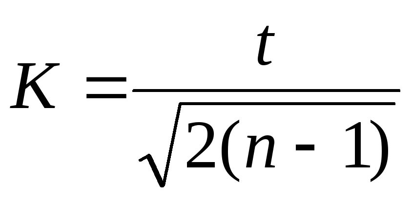
.

Knowing that with confidence probability R= 95% normalized deviation (Student's test at k =
)t = 1.960, let’s first calculate the value TO:

.

or 9.3%

or 12.3%

Thus, the general coefficient of variation with a 95% confidence level lies in the range from 9.3 to 12.3%. With repeated samples, the coefficient of variation will not exceed 12.3% and will not be below 9.3% in 95 cases out of 100.

Questions for self-control:

Problems for independent solution.

1. The average percentage of fat in milk during lactation of Kholmogory crossbred cows was as follows: 3.4; 3.6; 3.2; 3.1; 2.9; 3.7; 3.2; 3.6; 4.0; 3.4; 4.1; 3.8; 3.4; 4.0; 3.3; 3.7; 3.5; 3.6; 3.4; 3.8. Establish confidence intervals for the general mean at 95% confidence level (20 points).

2. On 400 hybrid rye plants, the first flowers appeared on average 70.5 days after sowing. The standard deviation was 6.9 days. Determine the error of the mean and confidence intervals for the general mean and variance at the significance level W= 0.05 and W= 0.01 (25 points).

3. When studying the length of leaves of 502 specimens of garden strawberries, the following data were obtained: = 7.86 cm; σ = 1.32 cm, =± 0.06 cm. Determine confidence intervals for the arithmetic population mean with significance levels of 0.01; 0.02; 0.05. (25 points).

4. In a study of 150 adult men, the average height was 167 cm, and σ = 6 cm. What are the limits of the general mean and general variance with a confidence probability of 0.99 and 0.95? (25 points).

5. The distribution of calcium in the blood serum of monkeys is characterized by the following selective indicators: = 11.94 mg%, σ = 1,27, n = 100. Construct a 95% confidence interval for the general mean of this distribution. Calculate the coefficient of variation (25 points).

6. The total nitrogen content in the blood plasma of albino rats at the age of 37 and 180 days was studied. The results are expressed in grams per 100 cm 3 of plasma. At the age of 37 days, 9 rats had: 0.98; 0.83; 0.99; 0.86; 0.90; 0.81; 0.94; 0.92; 0.87. At the age of 180 days, 8 rats had: 1.20; 1.18; 1.33; 1.21; 1.20; 1.07; 1.13; 1.12. Set confidence intervals for the difference at a confidence level of 0.95 (50 points).

7. Determine the boundaries of the 95% confidence interval for the general variance of the distribution of calcium (mg%) in the blood serum of monkeys, if for this distribution the sample size is n = 100, statistical error of the sample variance s σ 2 = 1.60 (40 points).

8. Determine the boundaries of the 95% confidence interval for the general variance of the distribution of 40 wheat spikelets along the length (σ 2 = 40.87 mm 2). (25 points).

9. Smoking is considered the main factor predisposing to obstructive pulmonary diseases. Passive smoking is not considered such a factor. Scientists doubted the harmlessness of passive smoking and examined the airway patency of non-smokers, passive and active smokers. To characterize the state of the respiratory tract, we took one of the indicators of external respiration function - the maximum volumetric flow rate of mid-expiration. A decrease in this indicator is a sign of airway obstruction. The survey data are shown in the table.

Using the table data, find 95% confidence intervals for the overall mean and overall variance for each group. What are the differences between the groups? Present the results graphically (25 points).

10. Determine the boundaries of the 95% and 99% confidence intervals for the general variance in the number of piglets in 64 farrows, if the statistical error of the sample variance s σ 2 = 8.25 (30 points).

11. It is known that the average weight of rabbits is 2.1 kg. Determine the boundaries of the 95% and 99% confidence intervals for the general mean and variance at n= 30, σ = 0.56 kg (25 points).

12. The grain content of the ear was measured for 100 ears ( X), ear length ( Y) and the mass of grain in the ear ( Z). Find confidence intervals for the general mean and variance at P 1 = 0,95, P 2 = 0,99, P 3 = 0.999 if = 19, = 6.766 cm, = 0.554 g; σ x 2 = 29.153, σ y 2 = 2. 111, σ z 2 = 0. 064. (25 points).

13. In 100 randomly selected ears of winter wheat, the number of spikelets was counted. The sample population was characterized by the following indicators: = 15 spikelets and σ = 2.28 pcs. Determine with what accuracy the average result was obtained ( ) and construct a confidence interval for the general mean and variance at 95% and 99% significance levels (30 points).

14. Number of ribs on fossil mollusk shells Orthambonites calligramma:

It is known that n = 19, σ = 4.25. Determine the boundaries of the confidence interval for the general mean and general variance at the significance level W = 0.01 (25 points).

15. To determine milk yield on a commercial dairy farm, the productivity of 15 cows was determined daily. According to data for the year, each cow gave on average the following amount of milk per day (l): 22; 19; 25; 20; 27; 17; thirty; 21; 18; 24; 26; 23; 25; 20; 24. Construct confidence intervals for the general variance and the arithmetic mean. Can we expect the average annual milk yield per cow to be 10,000 liters? (50 points).

16. In order to determine the average wheat yield for the agricultural enterprise, mowing was carried out on trial plots of 1, 3, 2, 5, 2, 6, 1, 3, 2, 11 and 2 hectares. Productivity (c/ha) from the plots was 39.4; 38; 35.8; 40; 35; 42.7; 39.3; 41.6; 33; 42; 29 respectively. Construct confidence intervals for the general variance and arithmetic mean. Can we expect that the average agricultural yield will be 42 c/ha? (50 points).